Technical Document

In September 2004, Dr. Ian D. Peggs, I-CORP INTERNATIONAL led Mark Powers and Jeff Blum of STS and Tim Ambrosius and Nick Sturzl (CQM) through the third (in-field) stage of the T-CLIC accreditation course for performing electrical liner integrity surveys. A half-day classroom session and a practical session in three test cells had previously been undergone at TRI.

The field test was performed on a new landfill cell consisting of a single HDPE geomembrane above clay with a cushion geotextile and 1 to 2 ft of drainage stone on top. The drainage stone had not been placed to the edge of the cell leaving an insulating gap at the edge of the geomembrane – the drainage stone was not in electrical contact with the subgrade clay, a necessary boundary condition for an effective survey. The only exception was at a haul road in one corner of the cell. A small sump in another corner of the cell was filled with water that was pumped to a hose to keep the stone and the top surface of the liner wet.

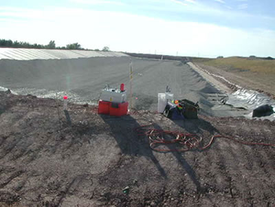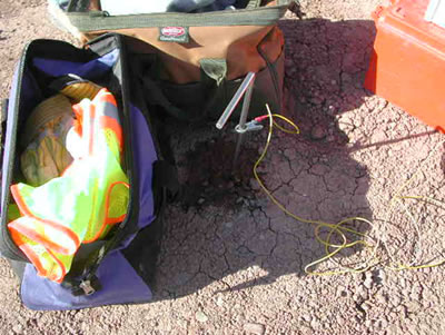
Test cell. Liner exposed around edge. Power supply (white) on top of red toolbox. Sump at right

Several interesting observations were made, making the session an extremely effective learning experienced:

• Initially no current was flowing between the current injector electrode (in the sump water) and the simulated calibration leak – 0.25 inches of exposed solid core wire – placed in the stone just above the liner.
• The calibration hole was buried further down in water standing on the liner – current flowed. Previously the calibration hole must have been in a void between the stones. But now there was no voltage reading between the survey probe electrodes on top of the stone.
• The calibration hole was moved to the sump water where there clearly would be no impediment to current flow and there would be no resistance between the applied potential electrodes and the survey probe electrodes. Initially there was still no reading from the survey probe but one soon appeared and remained. More on the reason why later.
• With all systems working correctly, a +/- 10 ft grid spacing was set up for 40 ft each side of the calibration leak, now buried under the drainage stone again. A parallel grid was established 10 ft to the side of the calibration hole.
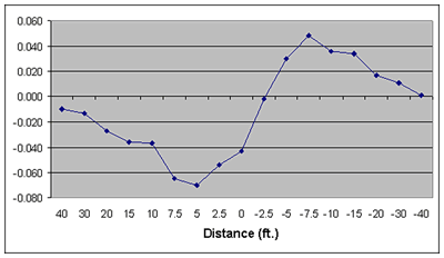
• The calibration hole was connected directly to the power supply, an optimistic situation, but one that should give a good leak indication signal. Figure 1 shows the survey potential profile for +/- 40 ft directly across the calibration hole obtained by one team. The typical up/down/up signal is evident, but is not very well defined. The maximum signal was about 6 V.

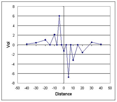Figure 1. Survey traverse across hole directly connected to power supply. “Reading” in volts. “Distance" in feet.

• The geometry of this signal can be more easily understood if one considers there to be a whirlpool directly above the leak and we are measuring the surface gradient on the water with a pair of probes. Away from the whirlpool the gradient is essentially zero. As the probe enters the whirlpool the slope increases to a maximum when the leading electrode is directly over the hole. When the probes are equidistant astride the hole there is no gradient. There is another maximum, but of the opposite sign to the previous one when the trailing electrode is directly over the hole. Then as the probe exits the whirlpool the gradient returns to zero. Such a signal can only occur at a hole.
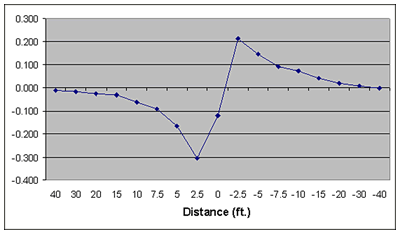
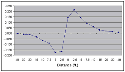
• In the real world the medium between the leak and he power supply is not a highly conductive copper wire, so the calibration hole was next connected to an electrode placed in the soil outside the liner approximately 150 ft from the current return electrode that was connected to the power supply. Thus we now simulate the real situation where there may be 150 ft between a real leak in the center of the cell and the current return electrode that can only be placed outside the cell. Figure 2a shows the +/- 40 ft survey obtained by the first team directly over the calibration hole – the characteristic signal is still evident but its amplitude is considerably decreased (250 mV). Even so the hole starts to be seen (> 3x background) at a distance of about 7.5 ft. Therefore, we could survey with a 10 ft grid spacing and easily see a hole the size of the calibration. In this orientation there will be no hole further than 5 ft from a measurement location.
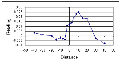
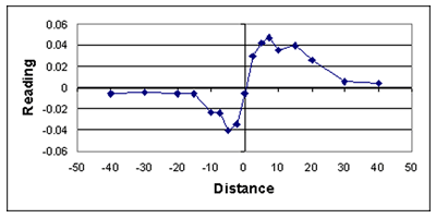
• The equivalent survey traverse made by the second team is shown in Figure 2b. This curve is much more well defined and at an applied voltage of only 50V (current 150 mA) detect the hole from a distance of 12.5 to 15 ft. The maximum signal is about 150 mV. When the applied potential was increased to 95 mV (and 250 mA) by Team 2 the maximum signal increased to about 250 mV, and the distance of detection increased marginally to about 15 ft, as shown in Figure 2c.

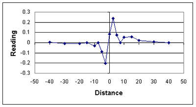Figure 2a. Survey across hole connected through ground to power supply

Figure 2b. As 2a but by Team 2 at 50 V (150 mA)

Figure 2c. As 2b but at 95 V (250 mA)

• When the survey is made 10 ft to the side of the hole the signal is, of course, lower (Figure 3a – Team 1)and probably is not high enough to use a grid spacing of 10 ft perpendicular to the previous orientation. At an applied voltage of 95 V Team 2 obtained similar results (Figure 3b)

Figure 3a. Survey 10 ft to side of hole. Team 1

Figure 3b. Survey 10 ft to side of hole. Team 2.

• Reducing the grid spacing to 5 ft generated an adequate signal (Figure 4a, Team 1, and Figure 4b, Team 2)

Figure 4a. Survey 5 ft to side of hole. Team 1

Figure 4b. Survey 5 ft to side of hole. Team 2.

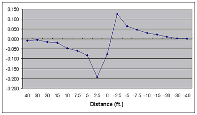
At 3 ft to the side the curve is much better defined (Figure 5, Team 2)

Figure 5. Survey 3 ft to side of hole. Team 2.

While it was generally felt that if the applied voltage was increased above 100 V, it would have been possible to detect the hole from a sideways distance of 10 ft. The teams decided to perform the production survey with a more conservative parallel grid spacing of 5 ft.

The major difference between the two teams was that Team 2 as more careful in making measurements at the prescribed distance which resulted in the better defined curves.

At one point during the calibration procedure it was noticed that the current had inexplicably dropped from about 250 mA to 50 mA. The current injection electrode in the stone drainage layer was checked; it had been buried in some wet sand in the rock for better contact conductance – nothing changed. The current return electrode in the soil outside the cell was examined and the soil appeared to be drying out and contracting from the electrode. The soil around the electrode was wetted and compacted against the electrode. The current was restored to its original value.

Electrode in drying ground must be watered to maintain good contact with ground.

Then during the production survey the measured signal was lost. The current was checked and found to be still high. The voltmeter was changed but no improvement occurred. There was adequate copper sulfate in the cells. The connections between the copper anodes in the cells and the terminals to the voltmeter were OK. However, the resistance between one of the electrode tips (that contact the rock) and the terminal to the voltmeter was high. The other was low. The dry deposits of rock dust were scraped off the electrode tips, the tips were soaked in copper sulfate for 10 minutes, and everything returned to normal. The survey continued. Clearly the same thing had happened at the start of the survey and was resolved by placing the probe electrodes in the sump water.

Clearly it is necessary to keep the ceramic tips soaked with copper sulfate, but this was the first time the tips have actually dried out for me during a survey.

The production survey continued towards the haul road where the signal started to increase significantly. A trench exposing the liner was dug across the haul road entrance and the signal returned to the previously normal value. Thus the haul road had been registering as a large leak with a signal that might swamp any signal from a nearby small leak in the liner.

Thus the calibration procedure and the production survey threw some interesting curves at the surveyors, but curves that enabled them (and me) to learn much about the characteristics of liner integrity surveys. Mark, Jeff, Tim, and Nick successfully gained their T-CLIC accreditations to perform liner integrity surveys.

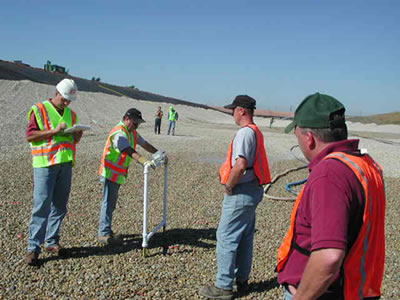Tim Ambrosius, Mark Powers, Jeff Blum, and Nick Sturzl starting survey.

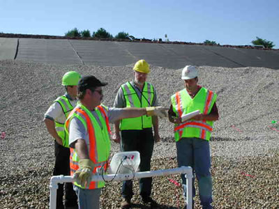Mark describing procedures to Bob Grefe (yellow hat) of Wisconsin DNR.

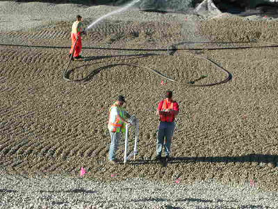Drainage stone must not be allowed to dry out.

To learn more about the T-CLIC Accreditation Course, please contact Ian Peggs.